How to Weigh a Supermassive Black Hole

At the center of every galaxy lies a black hole that's millions to billions the mass of our Sun. These supermassive black holes (SMBHs) are thought to play a crucial role in the formation and evolution of galaxies, and when we examine the properties of black holes and their host galaxies, we find that the two are deeply intertwined. In particular, the mass of SMBHs is strongly correlated with galaxy brightness and the velocity distribution of the galaxy's stars. At first this connection might seem obvious—black holes are known for their immense gravitational fields, so of course they're going to affect their hosts, right? Surprisingly, a SMBH's gravity can only control a miniscule region around it via gravity alone, a region known as the gravitational sphere of influence. The Milky Way's SMBH has a sphere of influence of only about 3 parsecs (~10 light years) in radius while the Milky Way itself is 5000 times larger at 15,000 parsecs.

So, how are the galaxy and black hole properties on such vastly different scales tied together? Maybe the black hole and the galaxy grow together from a common gas reservoir, so the black hole mass is simply a reflection of the galaxy's stellar mass. Maybe powerful jets and outflows, a byproduct of black hole growth, inject energy into the rest of the galaxy and regulate star formation. Maybe the coupling is purely statistical in nature with no direct physical connection between the two. All of these are plausible theories and each has broad implications for our understanding of how the Universe grows and evolves. Each predicts slightly different behavior for how the black hole-galaxy relations change over time, so if we can measure the black hole mass and galaxy properties precisely enough and over a long enough time period, we can rule out some theories and support others.

Fortunately, in astronomy, we can actually look back in time by observing more and more distant galaxies—since light travels at a finite speed, when we observe a galaxy, we're actually seeing a snapshot from when the light was emitted. For the most distant galaxies, this could be billions of years ago, allowing us to study the evolution of galaxies and black holes over nearly the entire 13.8 billion year history of the Universe.

Nearby, measuring black hole masses is relatively easy. We can study the motions of stars and gas within the black hole's sphere of influence region and calculate its mass from Kepler's laws. Far away, however, the sphere of influence is too small to resolve even with the most powerful telescopes. Instead, we can use a technique known as reverberation mapping, which is essentially a form of cosmic echolocation—similar to how bats emit sound waves to map their surroundings, we can use light emitted from near the black hole to map the surrounding gas. To fully understand reverberation mapping, we first need to understand some properties of light and how they relate to a special type of galaxy.

Light and its properties

Light behaves like a wave, similar to the waves you see on the surface of a pond, traveling outward from a source at a constant speed of 380,000 km/s (186,000 miles per second). The distance between the crests of the wave is called the wavelength, and is what determines the color we perceive when it reaches our eyes. The visible spectrum of light ranges from around 380 nm to 750 nm, with bluer light corresponding to the shorter wavelengths and redder light corresponding to the longer wavelengths.

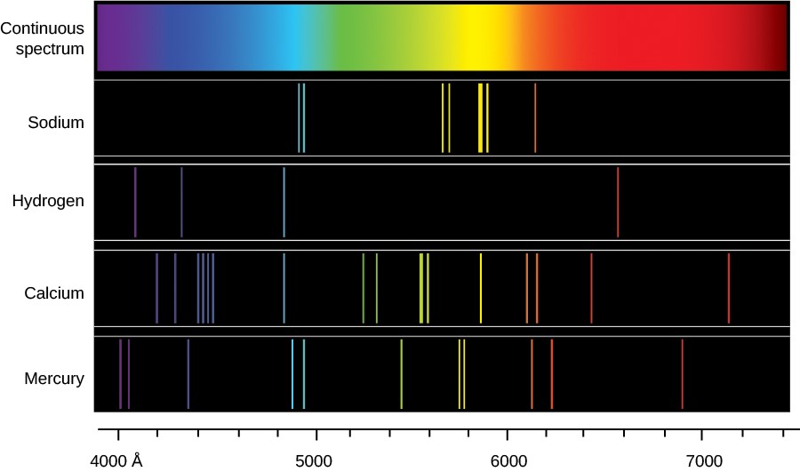
Some objects emit light across nearly all wavelengths of light in a continuum, such as the sun and incandescent light bulbs. You can see this in the smooth gradient of colors when you look at a rainbow or hold up a prism to a light bulb. Other objects, however, emit light at only a few specific wavelengths that are determined by the elements that make them up. These are called emission lines, and they appear as bright lines at specific wavelengths in a spectrum. Since the pattern of emission lines is unique to each element, they act as a sort of "fingerprint" that we can use to identify the chemical composition of objects. Fluorescent lights contain mercury and argon gas, so if you look at a fluorescent light through a prism, you'll see bright bands of light corresponding to those two elements. The image below shows an example of a smooth, continuous spectrum, as well as the emission line spectra of different elements.

Doppler Effect

Consider a source of light with an emission line at 580 nm that we perceive as yellow, and the source of light is moving towards an observer at near the speed of light (to the right in the animation below). Since the source is "catching up" to the emitted light, the waves get compressed in the direction of motion. Even though the source is emitting light at 580 nm, the observer will see the light as having a shorter wavelength. Shorter wavelengths are on the bluer end of the spectrum, so the light will be blueshifted relative to its actual emitted wavelength. On the other hand, if the source is moving away from the observer, the waves will be stretched out and the observer will perceive the light to be redder, or redshifted. This shift in wavelength is known as the Doppler effect. You've probably experienced the sound-wave version of the Doppler effect before when you've heard the pitch of an ambulance siren change as it passed by. In reality, the light-wave version is a bit more complicated and depends on Einstein's theory of relativity, but the basic idea is the same.

Since the wavelength of light we observe depends on the motion of the source towards or away from us, we can use the Doppler effect to measure a source's velocity relative to us. First, we use the known patterns of emission lines of different elements to identify some of our observed emission lines. Then, with our knowledge of the Doppler effect equations, we can calculate the velocity that would shift the emission lines to the wavelengths we observe.

An important thing to note is that the Doppler effect only applies to the component of the source's velocity that is along our line of sight. If the source is moving perpendicular to our line of sight (say, up or down in the animation above), then the observed wavelength will not be shifted. Therefore, we can only measure the component of the source's velocity that is directed towards or away from us, and we need to use other methods to measure any remaining velocity components.

Broad emission lines

Now, imagine our emission line source is orbiting around a massive object like a black hole. As the source is moving towards us, the light is blueshifted. As it moves away from us, it is redshifted.

Consider now a whole cloud of these sources, all emitting the same emission line. At any given moment, some of the clouds will be blueshifted, some will be redshifted, and others won't have any velocity component going towards or away from us to shift their light. If the cloud is far enough away, we won't be able to make out each individual source of light. Instead, the sources will be blurred together and we will observe the sum of all sources' individual contributions. Through a prism, the line will appear to be blurred out around the central wavelength rather than being a sharp peak. These are known as broad emission lines.

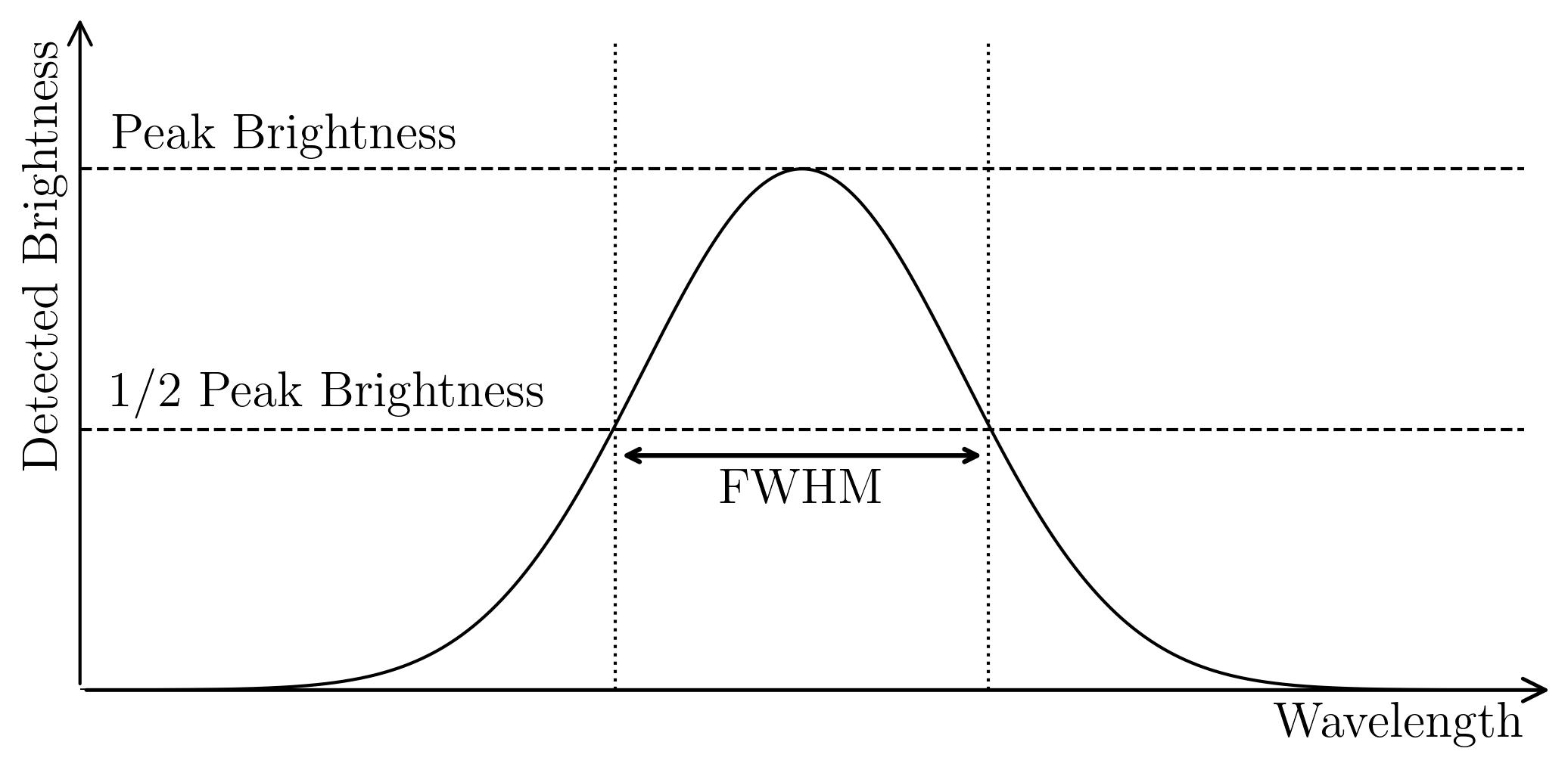
The width of the broad emission line can tell us about the velocities of the sources in the cloud—the faster they're moving, the broader the line will be. There are multiple ways to measure the emission line width, but the most common is the Full Width at Half Maximum, or FWHM. To measure the FWHM, you first measure how bright the emission line is at its peak. Then, you find the two wavelengths where the brightness is half of that peak brightness. The distance between these two wavelengths is the FWHM. Since we know the equations to convert wavelength shifts to velocities, the FWHM is usually reported as a velocity, $\Delta V_{\rm FWHM}$, in km/s. Note that the particles in the cloud might not all be moving at the same velocity, so $\Delta V_{\rm FWHM}$ should be considered an average or characteristic velocity.

Orbital motion equations

If we know the velocity, $v$, of a particle in orbit around a central massive object and the radius, $r$, of its orbit, we can calculate the central object's mass with the following equation: \begin{equation}\label{eq:mass_from_velocity} M = \frac{r v^2}{G}, \end{equation} where $G$ is the known gravitational constant equal to $6.674 \times 10^{-11} \, \text{m}^3 \, \text{kg}^{-1} \, \text{s}^{-2}$. In our cloud of line-emitting sources orbiting the central black hole, we saw that the FWHM of the broad emission line corresponds to the average velocity of the sources in the cloud. Similar to how each cloud has its own velocity, each also has its own radius, but we can consider an average radius of the whole cloud, $r_{\rm avg}$. With this information, we can plug in these values to calculate the black hole's mass: \begin{equation}\label{eq:mass_from_fwhm} M_{\rm BH} = \frac{r_{\rm avg} (\Delta V_{\rm FWHM})^2}{G}. \end{equation}

Active Galactic Nuclei

What we have in the BLR is similar to the rotating cloud of line-emitting sources we saw above with one important distinction: we don't know its size or geometry. It could be a disk, a torus, a sphere, or some other shape, and it could be oriented in any direction relative to us. BLRs of most AGNs only span a few microarcseconds (1 microarcsecond = 1/3,600,000,000th of a degree) on the sky, making it near-impossible to measure their size and shape directly with telescopes . This is where reverberation mapping comes in.

Reverberation Mapping

To determine the physical size of the BLR, we can take advantage of the fact that the speed of light is finite and takes time to travel from point A to point B. If you imagine a pulse of light emitted from the accretion disk, it will travel outwards in all directions. Some will travel towards us, the observer, and we will see it after a time, $t$, that depends on the distance from us to the galaxy. From that same pulse, some light will also travel out to clouds in the BLR where it will be absorbed and re-emitted as an emission line. That re-emitted light will also travel towards us, but it will arrive later than the continuum light pulse with a time lag, $\tau$. Since BLRs are typically a few light days to weeks in radius, the time lag is typically days to weeks as well, which is more than long enough for us to measure. This lag is illustrated in the animation below.

Of course, each point in the BLR will have a different time lag, depending on its distance from the accretion disk as well as its positioning along the $x$-axis. Points that are along our line of sight to the accretion disk will actually have no time lag. Regardless, multiplying the average time lags from all components of the BLR by the speed of light, $c$, gives a crude estimate of the size of the BLR: \begin{equation}\label{eq:blr_size} r_{\text{BLR}} \approx c \tau. \end{equation}

Measuring the Time Delay

AGNs don't send out pulses of light like in the animation above, but they do fluctuate in brightness over time. Therefore, if we continuously monitor an AGN, we should see the accretion disk continuum increase and decrease in brightness, and then see the broad emission lines follow the same brightness pattern after a time delay. This is precisely what's shown below. The blue points are measurements of the AGN continuum emission brightness over time. The orange points are measurements of the total brightness in the broad emission lines, which follow the same fluctuations as the continuum, but delayed by $\tau = 39.8$ days.

With our time delay in hand and our velocity estimate from the emission line width, we can combine Equations \eqref{eq:mass_from_fwhm} and \eqref{eq:blr_size} to get a final equation for the black hole mass. Since we're dealing with a lot of unknowns and making a lot of approximations (e.g. the unknown BLR geometry, using averages for BLR size, etc.), we'll add in a "fudge factor," $f$, to our equation: \begin{equation}\label{eq:bh_mass_fwhm} M_{\text{BH}} = f \cdot \frac{c \tau (\Delta V)^2}{G}. \end{equation} The value of $f$ is estimated to range from around 1 to 5 and is by far the most uncertain part of this equation, introducing a factor of $\sim$$2.5$ uncertainty in individual black hole mass measurements.

The Gold Standard: Modeling the Broad Line Region

So far, we've only been using the emission lines to measure their width and brightness. However, there's a wealth of additional information in the shape of the emission lines that can tell us more about the BLR structure. Going even further, precisely how the emission line shape responds to changes in the continuum brightness can tell us even more about the BLR. For instance, the bluer side of the emission line might respond faster than the redder side, or the central core might respond faster than the wings. If we can understand the BLR's structure, we can reduce the uncertainty black hole mass measurements by a factor of 2 or more. While this might not sound like much, these incremental improvements are necessary to make progress in our understanding of black hole-galaxy co-evolution.

The best way to extract all of this information is to create a full theoretical model of the BLR including its geometry, velocity distribution, and emission properties. We can then feed into the model the true continuum light curve that we observe and ask, "if this is the true BLR, what would the emission line look like at each point in time?" By comparing the model's predicted emission line to our actual measurements, we can adjust the model parameters until we find the best fit.

Below is an interactive tool that shows the CARAMEL model I used in my research. The region is modeled as a distributions of gas clouds, each represented as a single point in 3D space. There are several parameters that go into the model that can be adjusted with the sliders on the left. The top two panels show an edge-on view of the BLR where the observer is off to the right, and a face-on view which is what the observer would see if they had a powerful enough telescope. The middle-left panel shows the shape of the emission line profile that the BLR model would produce. The middle-right panel maps each individual BLR cloud to its time-lag and its line-of-sight velocity. The bottom panel shows the continuum brightness and overall broad emission line brightness over time. Finally, the box in the bottom-left gives the standard reverberation mapping measurements of the emission line FWHM and the measured time delay.

Real life results

In my PhD and postdoctoral research, I used this model to analyze the broad line region and measure supermassive black hole masses of 19 AGNs. One of the AGNs I analyzed is 21 billion light years away, and the light we observe from it was emitted 11.5 billion years ago . The Universe is only 13.8 billion years old, so when we observe this galaxy, we are looking the Universe in its infancy. The measurement of the black hole mass was among the most accurate made using reverberation mapping data with only 17% uncertainty, demonstrating that the modeling technique can yield precise measurements across the Universe's entire history.

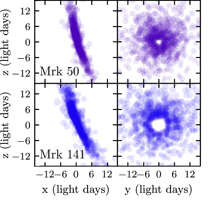
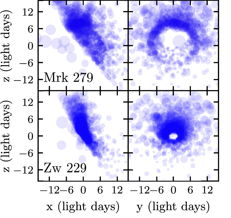
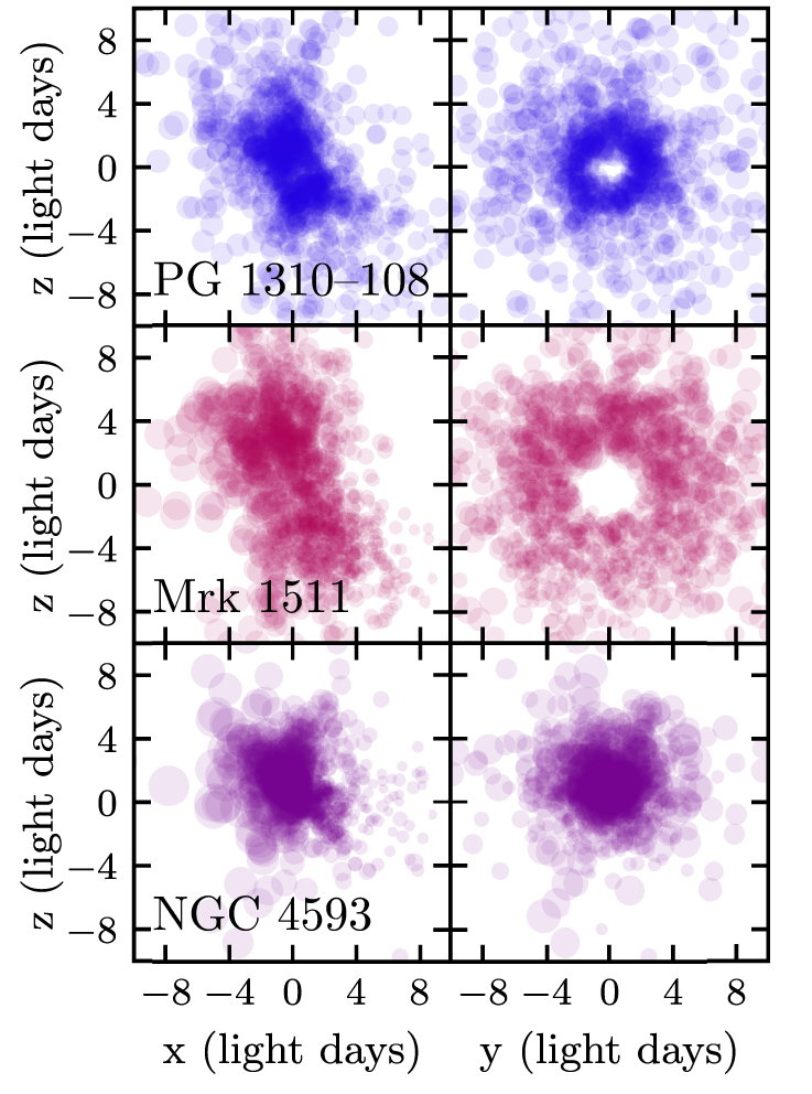
In addition to measuring black hole masses, we are also able to better understand the typical structure of the BLR and how it varies from galaxy to galaxy. The figure below shows the BLR models for seven of AGNs I studied as part of the Lick AGN Monitoring Project carried out at Lick Observatory. While there is some variation in the BLR structure, they all fit into the same general "thick disk with a hole" description.

These models are especially important because they allow us to better constrain the value of the fudge factor, $f$. The data required to fit these models is much more difficult to obtain than standard reverberation mapping data, so it is hard to do at scale. By building up a sample of BLRs where we do have modeling results, we can see how much $f$ varies from AGN to AGN and how it might depend on other properties we can observe. This would allow us to make improved $M_{\rm BH}$ measurements for the rest of the AGN population without needing to apply the full modeling approach, putting us one step closer to understanding our cosmological history.